python数据可视化制做带均线系统的移动平均线和边缘柱形图
AI 摘要 / TL;DR
python数据可视化制做带均线系统的移动平均线和边缘柱形图 来源: https://www.ucloud.cn/yun/130252.html 作者: 89542767 发布日期: 发布于2023 01 12 10:33 文中重要讲述了python数据可视化制做带均线系统的移动平均线和边缘柱形图,文章主题明确开展详细
来源: https://www.ucloud.cn/yun/130252.html 作者: 89542767 发布日期: 发布于2023-01-12 10:33
文中重要讲述了python数据可视化制做带均线系统的移动平均线和边缘柱形图,文章主题明确开展详细的简单介绍,具有极强的实际意义,需要的小伙伴可以学习下
一、制做带均线系统的移动平均线
实现方案:
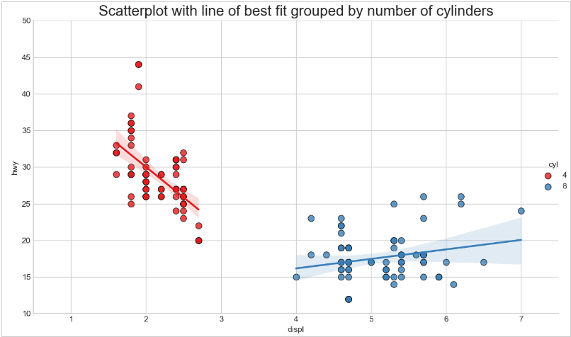
在移动平均线上再加上均线系统(线性拟合线)反映2个变量是正相关、反比或者无关联性。
进行编号:
在移动平均线上再加上均线系统(线性拟合线)反映2个变量是正相关、反比或者无关联性。蓝红2组数据信息各自设计出最理想的线性拟合线。
  import pandas as pd
  import matplotlib as mpl
  import matplotlib.pyplot as plt
  import seaborn as sns
  import warnings
  warnings.filterwarnings(action='once')
  plt.style.use('seaborn-whitegrid')
  sns.set_style("whitegrid")
  print(mpl.__version__)
  print(sns.__version__)
  def draw_scatter(file):
  #Import Data
  df=pd.read_csv(file)
  df_select=df.loc[df.cyl.isin([4,8]),:]
  #Plot
  gridobj=sns.lmplot(
  x="displ",
  y="hwy",
  hue="cyl",
  data=df_select,
  height=7,
  aspect=1.6,
  palette='Set1',
  scatter_kws=dict(s=60,linewidths=.7,edgecolors='black'))
  #Decorations
  sns.set(style="whitegrid",font_scale=1.5)
  gridobj.set(xlim=(0.5,7.5),ylim=(10,50))
  gridobj.fig.set_size_inches(10,6)
  plt.tight_layout()
  plt.title("Scatterplot with line of best fit grouped by number of cylinders")
  plt.show()
  draw_scatter("F:数据杂坛datasetsmpg_ggplot2.csv")
二、制做边缘柱形图
实现方案:
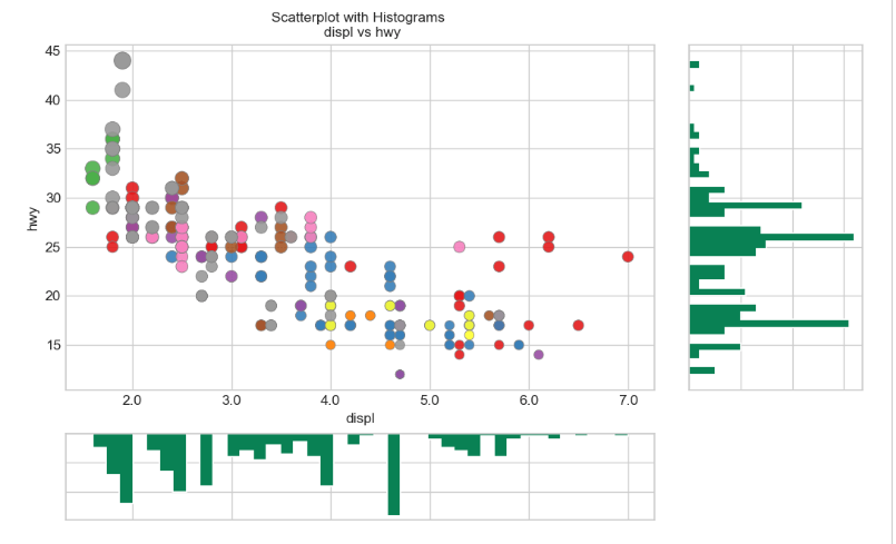
python制做边缘柱形图,用于呈现X和Y内在联系、及X和Y的单变量分布规律,主要运用于数据探索分析。
进行编号:
  import pandas as pd
  import matplotlib as mpl
  import matplotlib.pyplot as plt
  import seaborn as sns
  import warnings
  warnings.filterwarnings(action='once')
  plt.style.use('seaborn-whitegrid')
  sns.set_style("whitegrid")
  print(mpl.__version__)
  print(sns.__version__)
  def draw_Marginal_Histogram(file):
  #Import Data
  df=pd.read_csv(file)
  #Create Fig and gridspec
  fig=plt.figure(figsize=(10,6),dpi=100)
  grid=plt.GridSpec(4,4,hspace=0.5,wspace=0.2)
  #Define the axes
  ax_main=fig.add_subplot(grid[:-1,:-1])
  ax_right=fig.add_subplot(grid[:-1,-1],xticklabels=[],yticklabels=[])
  ax_bottom=fig.add_subplot(grid[-1,0:-1],xticklabels=[],yticklabels=[])
  #Scatterplot on main ax
  ax_main.scatter('displ',
  'hwy',
  s=df.cty*4,
  c=df.manufacturer.astype('category').cat.codes,
  alpha=.9,
  data=df,
  cmap="Set1",
  edgecolors='gray',
  linewidths=.5)
  #histogram on the right
  ax_bottom.hist(df.displ,
  40,
  histtype='stepfilled',
  orientation='vertical',
  color='#098154')
  ax_bottom.invert_yaxis()
  #histogram in the bottom
  ax_right.hist(df.hwy,
  40,
  histtype='stepfilled',
  orientation='horizontal',
  color='#098154')
  #Decorations
  ax_main.set(title='Scatterplot with Histogramsn displ vs hwy',
  xlabel='displ',
  ylabel='hwy')
  ax_main.title.set_fontsize(10)
  for item in([ax_main.xaxis.label,ax_main.yaxis.label]+
  ax_main.get_xticklabels()+ax_main.get_yticklabels()):
  item.set_fontsize(10)
  xlabels=ax_main.get_xticks().tolist()
  ax_main.set_xticklabels(xlabels)
  plt.show()
  draw_Marginal_Histogram("F:数据杂坛datasetsmpg_ggplot2.csv")
综上所述,这篇文章就给大家介绍到这里了,希望可以给大家带来帮助。