如何使用注意力模型生成图像描述？

摘要：本教程中用到了基于注意力的模型，它使我们很直观地看到当文字生成时模型会关注哪些部分。运行的时候，它会自动下载数据集，使用模型训练一个编码解码器，然后用模型对新图像进行文字描述。

图像描述类任务就是给图像生成一个标题。 给定一个图像：

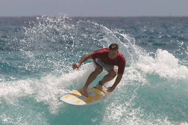
图片出处, 许可证：公共领域

我们的目标是用一句话来描述图片， 比如「一个冲浪者正在冲浪」。 本教程中用到了基于注意力的模型，它使我们很直观地看到当文字生成时模型会关注哪些部分。 

这个模型的结构类似于论文： Show, Attend and Tell: Neural Image Caption Generation with Visual Attention.（https://arxiv.org/abs/1502.03044）

本教程中的代码使用到了  tf.keras （https://www.tensorflow.org/guide/keras） 和  eager execution （https://www.tensorflow.org/programmers_guide/eager）这两个工具，链接里有详细的内容可以学习。

这个 notebook 展示了一个端到端模型。 运行的时候，它会自动下载 MS-COCO （http://cocodataset.org/#home）数据集，使用 Inception V3 模型训练一个编码 - 解码器，然后用模型对新图像进行文字描述。

这篇代码可以在 Colab （https://colab.research.google.com/github/tensorflow/tensorflow/blob/master/tensorflow/contrib/eager/python/examples/generative_examples/image_captioning_with_attention.ipynb） 中运行，但是需要 TensorFlow 的版本 >=1.9   

本实验对数据进行打乱以后取前 30000 篇描述作为训练集，对应 20000 篇图片（一张图片可能会包含多个描述）。 训练模型的数据量相对较小，因此只用了一个 P100 GPU，训练模型大约需要两个小时。

# Import TensorFlow and enable eager execution

# This code requires TensorFlow version >=1.9

import tensorflow as tf

tf.enable_eager_execution()

# We"ll generate plots of attention in order to see which parts of an image

# our model focuses on during captioning

import matplotlib.pyplot as plt

# Scikit-learn includes many helpful utilities

from sklearn.model_selection import train_test_split

from sklearn.utils import shuffle

import re

import numpy as np

import os

import time

import json

from glob import glob

from PIL import Image

import pickle

下载 MS-COCO 数据集

MS-COCO （http://cocodataset.org/#home）数据集包含 82,000 多张图片，每张图片都是用至少 5 句不同的文字描述的。 下面的代码在运行时会自动下载并且解压数据。

注意： 提前下载好数据，数据文件大小 13GB 。

annotation_zip = tf.keras.utils.get_file("captions.zip", 

                                         cache_subdir=os.path.abspath("."),

                                         origin = "http://images.cocodataset.org/annotations/annotations_trainval2014.zip",

                                         extract = True)

annotation_file = os.path.dirname(annotation_zip)+"/annotations/captions_train2014.json"

name_of_zip = "train2014.zip"

if not os.path.exists(os.path.abspath(".") + "/" + name_of_zip):

 image_zip = tf.keras.utils.get_file(name_of_zip, 

                                     cache_subdir=os.path.abspath("."),

                                     origin = "http://images.cocodataset.org/zips/train2014.zip",

                                     extract = True)

 PATH = os.path.dirname(image_zip)+"/train2014/"

else:

 PATH = os.path.abspath(".")+"/train2014/"

选择是否压缩训练集大小来减少训练时间

本教程中选择用 30000 篇描述和它们对应的图片来训练模型，但是当使用更多数据时，实验结果的质量通常会得到提高。

# read the json file

with open(annotation_file, "r") as f:

   annotations = json.load(f)

# storing the captions and the image name in vectors

all_captions = []

all_img_name_vector = []

for annot in annotations["annotations"]:

   caption = " " + annot["caption"] + " "

   image_id = annot["image_id"]

   full_coco_image_path = PATH + "COCO_train2014_" + "%012d.jpg" % (image_id)

   all_img_name_vector.append(full_coco_image_path)

   all_captions.append(caption)

# shuffling the captions and image_names together

# setting a random state

train_captions, img_name_vector = shuffle(all_captions,

                                         all_img_name_vector,

                                         random_state=1)

# selecting the first 30000 captions from the shuffled set

num_examples = 30000

train_captions = train_captions[:num_examples]

img_name_vector = img_name_vector[:num_examples]

len(train_captions), len(all_captions)

Inceptions v3 图像预处理

这个步骤中需要使用 InceptionV3 （在 Imagenet 上训练好的模型） 对每一张图片进行分类，并且从最后一个卷积层中提取特征。

首先，我们需要将图像转换为 inceptionV3 需要的格式：

把图像的大小固定到 （299, 299）

使用 preprocess_input （https://www.tensorflow.org/api_docs/python/tf/keras/applications/inception_v3/preprocess_input）函数将像素调整到 -1 到 1 的范围内（为了匹配 inceptionV3 的输入格式）。

def load_image(image_path):

   img = tf.read_file(image_path)

   img = tf.image.decode_jpeg(img, channels=3)

   img = tf.image.resize_images(img, (299, 299))

   img = tf.keras.applications.inception_v3.preprocess_input(img)

   return img, image_path

初始化 InceptionV3 & 下载 Imagenet 的预训练权重

将 InceptionV3 的最后一个卷积层作为输出层时，需要创建一个 keras 模型。

将处理好的图片输入神经网络，然后提取最后一层中获得的向量作为图像特征保存成字典格式（图名 --> 特征向量）；

选择卷积层的目的是为了更好地利用注意力机制，并且输出层的数据大小是8x8x2048；

为了提高模型质量的瓶颈，不要在预训练的时候添加注意力机制；

在网络中训练完成以后，将缓存的字典文件输出为 pickle 文件并且保存到本地磁盘。

image_model = tf.keras.applications.InceptionV3(include_top=False, 

                                               weights="imagenet")

new_input = image_model.input

hidden_layer = image_model.layers[-1].output

image_features_extract_model = tf.keras.Model(new_input, hidden_layer)

保存从 InceptionV3中提取的特征

利用 InceptionV3 对图像进行预处理以后将输出保存到本地磁盘，将输出缓存到 RAM 中会更快，但是内存更密集，每张图片都需要 8 * 8 * 2048 浮点数大小。 在写入时，这个大小可能会超过 Colab 的限制（也许会有浮动，但是当前这个实例显示大约需要 12GB）。

采用更复杂的缓存策略可以提高性能，但前提是代码会更的更复杂。例如，通过对数据进行分区来减少磁盘的随机访问 I/O 。

通过 GPU 在 Colab 上运行这个模型大约需要花费 10 分钟。假如需要直观地看程序进度，可以安装 tqdm (!pip install tqdm)， 并且修改这一行代码：

for img, path in image_dataset: 为：for img, path in tqdm(image_dataset):

# getting the unique images

encode_train = sorted(set(img_name_vector))

# feel free to change the batch_size according to your system configuration

image_dataset = tf.data.Dataset.from_tensor_slices(

                               encode_train).map(load_image).batch(16)

for img, path in image_dataset:

 batch_features = image_features_extract_model(img)

 batch_features = tf.reshape(batch_features, 

                             (batch_features.shape[0], -1, batch_features.shape[3]))

 for bf, p in zip(batch_features, path):

   path_of_feature = p.numpy().decode("utf-8")

   np.save(path_of_feature, bf.numpy())

对描述文字的预处理

首先，我们需要对描述进行分词，英文等西语可以按空格分词。分词以后得到一个包括所有词的词表（不重复）；

然后，只保存词表中的前 5000 个词， 其他的词标记为 "UNK" (不认识的词)；

最后，创建「词-编号」和「编号-词」的索引表；

最后将最长的一个句子作为所有句子的向量长度。

# This will find the maximum length of any caption in our dataset

def calc_max_length(tensor):

   return max(len(t) for t in tensor)

# The steps above is a general process of dealing with text processing

# choosing the top 5000 words from the vocabulary

top_k = 5000

tokenizer = tf.keras.preprocessing.text.Tokenizer(num_words=top_k, 

                                                 oov_token="", 

                                                 filters="!"#$%&()*+.,-/:;=?@[]^_`{|}~ ")

tokenizer.fit_on_texts(train_captions)

train_seqs = tokenizer.texts_to_sequences(train_captions)

tokenizer.word_index = {key:value for key, value in tokenizer.word_index.items() if value <= top_k}

# putting token in the word2idx dictionary

tokenizer.word_index[tokenizer.oov_token] = top_k + 1

tokenizer.word_index[""] = 0

# creating the tokenized vectors

train_seqs = tokenizer.texts_to_sequences(train_captions)

# creating a reverse mapping (index -> word)

index_word = {value:key for key, value in tokenizer.word_index.items()}

# padding each vector to the max_length of the captions

# if the max_length parameter is not provided, pad_sequences calculates that automatically

cap_vector = tf.keras.preprocessing.sequence.pad_sequences(train_seqs, padding="post")

# calculating the max_length 

# used to store the attention weights

max_length = calc_max_length(train_seqs)

将数据分为训练集和测试集

# Create training and validation sets using 80-20 split

img_name_train, img_name_val, cap_train, cap_val = train_test_split(img_name_vector, 

                                                                   cap_vector, 

                                                                   test_size=0.2, 

                                                                   random_state=0)

len(img_name_train), len(cap_train), len(img_name_val), len(cap_val)

准备好图形和描述数据后，就可以用 tf.data 训练集来训练模型了！

# feel free to change these parameters according to your system"s configuration

BATCH_SIZE = 64

BUFFER_SIZE = 1000

embedding_dim = 256

units = 512

vocab_size = len(tokenizer.word_index)

# shape of the vector extracted from InceptionV3 is (64, 2048)

# these two variables represent that

features_shape = 2048

attention_features_shape = 64

# loading the numpy files 

def map_func(img_name, cap):

   img_tensor = np.load(img_name.decode("utf-8")+".npy")

   return img_tensor, cap

dataset = tf.data.Dataset.from_tensor_slices((img_name_train, cap_train))

# using map to load the numpy files in parallel

# NOTE: Be sure to set num_parallel_calls to the number of CPU cores you have

# https://www.tensorflow.org/api_docs/python/tf/py_func

dataset = dataset.map(lambda item1, item2: tf.py_func(

         map_func, [item1, item2], [tf.float32, tf.int32]), num_parallel_calls=8)

# shuffling and batching

dataset = dataset.shuffle(BUFFER_SIZE)

# https://www.tensorflow.org/api_docs/python/tf/contrib/data/batch_and_drop_remainder

dataset = dataset.batch(BATCH_SIZE)

dataset = dataset.prefetch(1)

模型结构

有趣的是，本实验中的解码器与 Neural Machine Translation with Attention （https://github.com/tensorflow/tensorflow/blob/master/tensorflow/contrib/eager/python/examples/nmt_with_attention/nmt_with_attention.ipynb）这篇论文中的结构完全相同。

这个模型的结构参考了 Show, Attend and Tell （https://arxiv.org/pdf/1502.03044.pdf）这篇文章。

在本教程的实验中，我们从 InceptionV3 模型的下卷积层中提取特征，特征向量的大小为 (8, 8, 2048)；

需要把这个形状拉伸到 (64, 2048)；

把这个向量输入到 CNN 编码器(还包括了一个全连接层)；

用 RNN (这里用的是 RNN 的改进算法 GRU) 来预测词序列。

def gru(units):

 # If you have a GPU, we recommend using the CuDNNGRU layer (it provides a 

 # significant speedup).

 if tf.test.is_gpu_available():

   return tf.keras.layers.CuDNNGRU(units, 

                                   return_sequences=True, 

                                   return_state=True, 

                                   recurrent_initializer="glorot_uniform")

 else:

   return tf.keras.layers.GRU(units, 

                              return_sequences=True, 

                              return_state=True, 

                              recurrent_activation="sigmoid", 

                              recurrent_initializer="glorot_uniform")

class BahdanauAttention(tf.keras.Model):

 def __init__(self, units):

   super(BahdanauAttention, self).__init__()

   self.W1 = tf.keras.layers.Dense(units)

   self.W2 = tf.keras.layers.Dense(units)

   self.V = tf.keras.layers.Dense(1)

 def call(self, features, hidden):

   # features(CNN_encoder output) shape == (batch_size, 64, embedding_dim)

   # hidden shape == (batch_size, hidden_size)

   # hidden_with_time_axis shape == (batch_size, 1, hidden_size)

   hidden_with_time_axis = tf.expand_dims(hidden, 1)

   # score shape == (batch_size, 64, hidden_size)

   score = tf.nn.tanh(self.W1(features) + self.W2(hidden_with_time_axis))

   # attention_weights shape == (batch_size, 64, 1)

   # we get 1 at the last axis because we are applying score to self.V

   attention_weights = tf.nn.softmax(self.V(score), axis=1)

   # context_vector shape after sum == (batch_size, hidden_size)

   context_vector = attention_weights * features

   context_vector = tf.reduce_sum(context_vector, axis=1)

   return context_vector, attention_weights

class BahdanauAttention(tf.keras.Model):

 def __init__(self, units):

   super(BahdanauAttention, self).__init__()

   self.W1 = tf.keras.layers.Dense(units)

   self.W2 = tf.keras.layers.Dense(units)

   self.V = tf.keras.layers.Dense(1)

 def call(self, features, hidden):

   # features(CNN_encoder output) shape == (batch_size, 64, embedding_dim)

   # hidden shape == (batch_size, hidden_size)

   # hidden_with_time_axis shape == (batch_size, 1, hidden_size)

   hidden_with_time_axis = tf.expand_dims(hidden, 1)

   # score shape == (batch_size, 64, hidden_size)

   score = tf.nn.tanh(self.W1(features) + self.W2(hidden_with_time_axis))

   # attention_weights shape == (batch_size, 64, 1)

   # we get 1 at the last axis because we are applying score to self.V

   attention_weights = tf.nn.softmax(self.V(score), axis=1)

   # context_vector shape after sum == (batch_size, hidden_size)

   context_vector = attention_weights * features

   context_vector = tf.reduce_sum(context_vector, axis=1)

   return context_vector, attention_weights

class CNN_Encoder(tf.keras.Model):

   # Since we have already extracted the features and dumped it using pickle

   # This encoder passes those features through a Fully connected layer

   def __init__(self, embedding_dim):

       super(CNN_Encoder, self).__init__()

       # shape after fc == (batch_size, 64, embedding_dim)

       self.fc = tf.keras.layers.Dense(embedding_dim)

   def call(self, x):

       x = self.fc(x)

       x = tf.nn.relu(x)

       return x

class RNN_Decoder(tf.keras.Model):

 def __init__(self, embedding_dim, units, vocab_size):

   super(RNN_Decoder, self).__init__()

   self.units = units

   self.embedding = tf.keras.layers.Embedding(vocab_size, embedding_dim)

   self.gru = gru(self.units)

   self.fc1 = tf.keras.layers.Dense(self.units)

   self.fc2 = tf.keras.layers.Dense(vocab_size)

   self.attention = BahdanauAttention(self.units)

 def call(self, x, features, hidden):

   # defining attention as a separate model

   context_vector, attention_weights = self.attention(features, hidden)

   # x shape after passing through embedding == (batch_size, 1, embedding_dim)

   x = self.embedding(x)

   # x shape after concatenation == (batch_size, 1, embedding_dim + hidden_size)

   x = tf.concat([tf.expand_dims(context_vector, 1), x], axis=-1)

   # passing the concatenated vector to the GRU

   output, state = self.gru(x)

   # shape == (batch_size, max_length, hidden_size)

   x = self.fc1(output)

   # x shape == (batch_size * max_length, hidden_size)

   x = tf.reshape(x, (-1, x.shape[2]))

   # output shape == (batch_size * max_length, vocab)

   x = self.fc2(x)

   return x, state, attention_weights

 def reset_state(self, batch_size):

   return tf.zeros((batch_size, self.units))

encoder = CNN_Encoder(embedding_dim)

decoder = RNN_Decoder(embedding_dim, units, vocab_size)

optimizer = tf.train.AdamOptimizer()

# We are masking the loss calculated for padding

def loss_function(real, pred):

   mask = 1 - np.equal(real, 0)

   loss_ = tf.nn.sparse_softmax_cross_entropy_with_logits(labels=real, logits=pred) * mask

   return tf.reduce_mean(loss_)

训练

提取  .npy 相关的文件中存储的特征并输入到编码器中去；

将编码器的输出、隐状态（初始化为 0） 和解码器的输入（句子分词结果的索引集合） 一起输入到解码器中去；

解码器返回预测结果和隐向量；

然后把解码器输出的隐向量传回模型，预测结果需用于计算损失函数；

使用 teacher forcing 来决定解码器的下一个输入；

Teacher forcing 是用于筛选编码器下一个输入词的技术；

最后一步是计算梯度，用于进行反向传递以最小化损失函数值。

# adding this in a separate cell because if you run the training cell 

# many times, the loss_plot array will be reset

loss_plot = []

EPOCHS = 20

for epoch in range(EPOCHS):

   start = time.time()

   total_loss = 0

   for (batch, (img_tensor, target)) in enumerate(dataset):

       loss = 0

       # initializing the hidden state for each batch

       # because the captions are not related from image to image

       hidden = decoder.reset_state(batch_size=target.shape[0])

       dec_input = tf.expand_dims([tokenizer.word_index[""]] * BATCH_SIZE, 1)

       with tf.GradientTape() as tape:

           features = encoder(img_tensor)

           for i in range(1, target.shape[1]):

               # passing the features through the decoder

               predictions, hidden, _ = decoder(dec_input, features, hidden)

               loss += loss_function(target[:, i], predictions)

               # using teacher forcing

               dec_input = tf.expand_dims(target[:, i], 1)

       total_loss += (loss / int(target.shape[1]))

       variables = encoder.variables + decoder.variables

       gradients = tape.gradient(loss, variables) 

       optimizer.apply_gradients(zip(gradients, variables), tf.train.get_or_create_global_step())

       if batch % 100 == 0:

           print ("Epoch {} Batch {} Loss {:.4f}".format(epoch + 1, 

                                                         batch, 

                                                         loss.numpy() / int(target.shape[1])))

   # storing the epoch end loss value to plot later

   loss_plot.append(total_loss / len(cap_vector))

   print ("Epoch {} Loss {:.6f}".format(epoch + 1, 

                                        total_loss/len(cap_vector)))

   print ("Time taken for 1 epoch {} sec ".format(time.time() - start))

plt.plot(loss_plot)

plt.xlabel("Epochs")

plt.ylabel("Loss")

plt.title("Loss Plot")

plt.show()

注意事项

评价函数与迭代训练的过程类似，除了不使用 teacher forcing 机制，解码器的每一步输入都是前一步的预测结果、编码器输入和隐状态；

当模型预测到最后一个词时停止；

在每一步存储注意力层的权重的权重。

def evaluate(image):

   attention_plot = np.zeros((max_length, attention_features_shape))

   hidden = decoder.reset_state(batch_size=1)

   temp_input = tf.expand_dims(load_image(image)[0], 0)

   img_tensor_val = image_features_extract_model(temp_input)

   img_tensor_val = tf.reshape(img_tensor_val, (img_tensor_val.shape[0], -1, img_tensor_val.shape[3]))

   features = encoder(img_tensor_val)

   dec_input = tf.expand_dims([tokenizer.word_index[""]], 0)

   result = []

   for i in range(max_length):

       predictions, hidden, attention_weights = decoder(dec_input, features, hidden)

       attention_plot[i] = tf.reshape(attention_weights, (-1, )).numpy()

       predicted_id = tf.multinomial(tf.exp(predictions), num_samples=1)[0][0].numpy()

       result.append(index_word[predicted_id])

       if index_word[predicted_id] == "":

           return result, attention_plot

       dec_input = tf.expand_dims([predicted_id], 0)

   attention_plot = attention_plot[:len(result), :]

   return result, attention_plot

def plot_attention(image, result, attention_plot):

   temp_image = np.array(Image.open(image))

   fig = plt.figure(figsize=(10, 10))

   len_result = len(result)

   for l in range(len_result):

       temp_att = np.resize(attention_plot[l], (8, 8))

       ax = fig.add_subplot(len_result//2, len_result//2, l+1)

       ax.set_title(result[l])

       img = ax.imshow(temp_image)

       ax.imshow(temp_att, cmap="gray", alpha=0.6, extent=img.get_extent())

   plt.tight_layout()

   plt.show()

# captions on the validation set

rid = np.random.randint(0, len(img_name_val))

image = img_name_val[rid]

real_caption = " ".join([index_word[i] for i in cap_val[rid] if i not in [0]])

result, attention_plot = evaluate(image)

print ("Real Caption:", real_caption)

print ("Prediction Caption:", " ".join(result))

plot_attention(image, result, attention_plot)

# opening the image

Image.open(img_name_val[rid])

使用自己的数据集进行训练

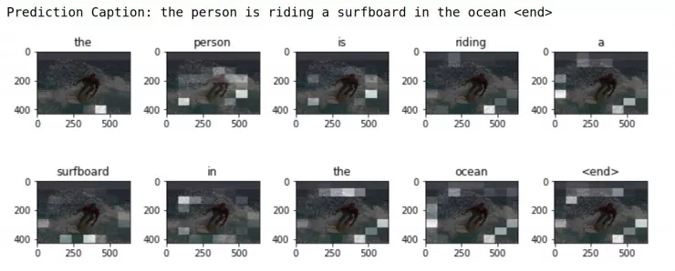
为了让这个实验更有趣，下面提供了方法可以让你用自己的图片测试刚刚训练好的模型进行图片描述。但是需要注意，这个模型用的数据相对较少，假设你的图片和训练集区别太大，可能会出现比较奇怪的结果。

image_url = "https://tensorflow.org/images/surf.jpg"

image_extension = image_url[-4:]

image_path = tf.keras.utils.get_file("image"+image_extension, 

                                    origin=image_url)

result, attention_plot = evaluate(image_path)

print ("Prediction Caption:", " ".join(result))

plot_attention(image_path, result, attention_plot)

# opening the image

Image.open(image_path)

下一步计划

恭喜你！已经可以训练一个基于注意力机制的图片描述模型，而且你也可以尝试对不同的图像数据集进行实验。有兴趣的话，可以看一下这个示例 ： Neural Machine Translation with Attention（https://github.com/tensorflow/tensorflow/blob/master/tensorflow/contrib/eager/python/examples/nmt_with_attention/nmt_with_attention.ipynb）。 这个机器翻译模型与本实验使用的结构相似，可以翻译西班牙语和英语句子。

原文链接：

https://colab.research.google.com/github/tensorflow/tensorflow/blob/master/tensorflow/contrib/eager/python/examples/generative_examples/image_captioning_with_attention.ipynb#scrollTo=io7ws3ReRPGv

声明：文章收集于网络，如有侵权，请联系小编及时处理，谢谢！

商业智能与数据分析群

兴趣范围包括各种让数据产生价值的办法，实际应用案例分享与讨论，分析工具，ETL工具，数据仓库，数据挖掘工具，报表系统等全方位知识

QQ群：81035754